Using the Backward Compatibility ML Compatibility Analysis Widget

Note

At the moment, the Compatibility Analysis Widget only works with PyTorch models. If you are interested in using the widget with TensorFlow, please let us know by submitting a Feature request.

The compatibility analysis widget can be used to quickly determine which loss function and value of λ_c performs best for your models. The widget will train a new model h2 using backward compatibility loss functions of your choice. Refer to Integrating the Backward Compatibility ML Loss Functions to see a list of the loss functions that are available. The widget will train h2 several times with different values of λ_c and show a visualization of the results. We will discuss how to use the CompatibilityAnalysis API and how to interpret the resulting visualizations.

How to Use the CompatibilityAnalysis API

The CompatibilityAnalysis API has a large number of parameters. To view the Python documentation for the API, execute ?CompatibilityAnalysis within a Jupyter notebook. The documentation for all of the parameters will be displayed at the bottom of the window.

In this article, we will reference the compatibility-analysis-cifar10-resnet18 example notebook. You can find this notebook at ./examples/compatibility-analysis-cifar10-resnet18 from the BackwardCompatibilityML project root. This notebook uses the widget to compare the performance of resnet18 with the following six-layer network using the cifar10 dataset:

class Net(nn.Module):

    def __init__(self):
        super().__init__()
        self.conv1 = nn.Conv2d(3, 18, kernel_size=3, stride=1, padding=1)
        self.fc2 = nn.Linear(18*32*32, 192)
        self.fc3 = nn.Linear(192, 192)
        self.fc4 = nn.Linear(192, 192)
        self.fc5 = nn.Linear(192, 192)
        self.fc6 = nn.Linear(192, 10)

    def forward(self, x):
        x = F.relu(self.conv1(x))
        x = x.view(-1, 18*32*32)
        x = F.relu(self.fc2(x))
        x = F.relu(self.fc3(x))
        x = F.relu(self.fc4(x))
        x = F.relu(self.fc5(x))
        x = self.fc6(x)

        return x, F.softmax(x, dim=1), F.log_softmax(x, dim=1)

The last cell in the notebook instantiates the widget:

analysis = CompatibilityAnalysis("sweeps-cifar10", 5, h1, h2, train_loader, test_loader,
    batch_size_train, batch_size_test,
    OptimizerClass=optim.SGD,
    optimizer_kwargs={"lr": learning_rate, "momentum": momentum},
    NewErrorLossClass=bcloss.BCCrossEntropyLoss,
    StrictImitationLossClass=bcloss.StrictImitationCrossEntropyLoss,
    lambda_c_stepsize=0.50,
    get_instance_image_by_id=get_instance_image,
    device="cuda")

Here, h1 refers to the resnet18 model, and h2 refers to the simple Net model. train_loader and test_loader are the train and test datasets. The BCCrossEntropyLoss and StrictImitationCrossEntropyLoss loss functions will be used to train h2. lambda_c_stepsize has been set to a relatively large value of 0.50 to reduce runtime. The number of samples of λ_c in the sweep is inversely proportional to lambda_c_stepsize. In other words, if lambda_c_stepsize is small, then the sweep will compute many samples, many points will be shown in the scatter plot, and the sweep will take longer to finish. Finally, the device has been set to cuda. It should be set to cpu if you do not have a GPU in your machine.

Interpreting the Visualizations

The first time the CompatibilityAnalysis widget is run, only a Start Sweep button will be shown. Click on it to start the sweep. The sweep will likely take several minutes to run. When it is complete, the widget will plot the results. The following screenshot shows the results from the compatibility-analysis-cifar10-resnet18 example notebook.

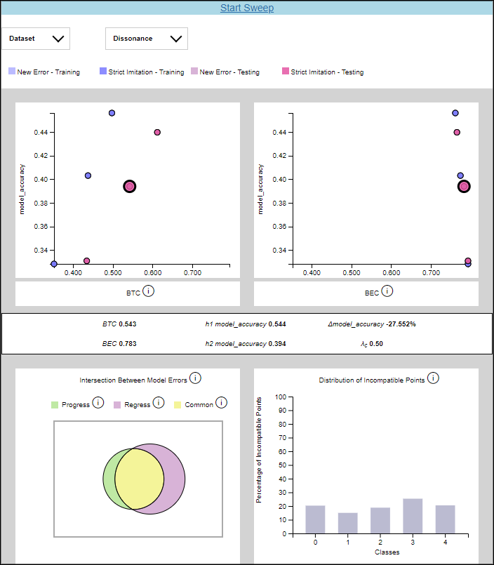
The drop-down menus contain options to filter the data shown in the scatter plots. The Dataset drop-down has options for selecting the training or testing set data. The Dissonance drop-down has options for selecting the New Error or Strict Imitation loss functions.

The two scatter plots graph the backward compatibility of the model against the model accuracy for a particular value of λ_c. Hovering over a point shows the value of λ_c for that point. Clicking on a point loads detailed results and error analysis for that particular value of λ_c.

The numeric values for BTC, BEC, model accuracy, and λ_c are shown in a table in the middle of the widget. Below that table, there is a Venn diagram and a histogram that plot the errors made by each model. The Venn diagram shows the intersection of errors made by the previous model with errors made by the new model. The red region represents errors made only by the new model, the yellow region represents errors made by both models, and the green region represents errors made only by the old model. The histogram breaks down incompatible data points by class. A point is considered incompatible if it was classified correctly by the old model but incorrectly by the new model. Note that the histogram is paginated with five classes shown per page.

The bars on the histogram and regions of the Venn diagram are clickable. When clicked, the data instances that have been misclassified will be displayed in a table at the bottom of the widget. This table is useful for exploring the dataset to determine why the models are misclassifying the data.

In the example below, class 0 has been selected in the histogram. The mislabeled pictures are shown in the table underneath. Notice that h1’s predictions match the ground truth for each data point while h2’s predictions do not. This is what we would expect to see based on our definition of incompatible points.

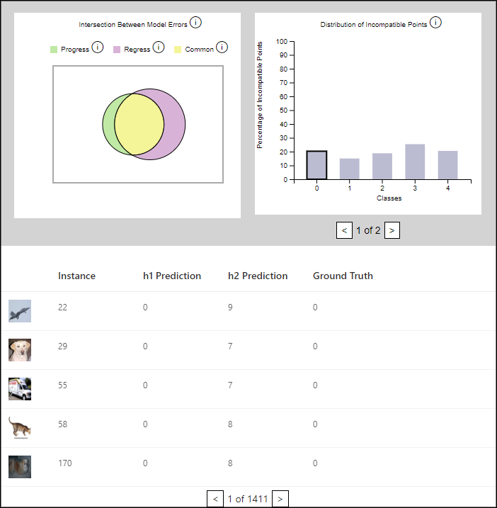
The CompatibilityAnalysis API contains two optional parameters, get_instance_metadata and get_instance_image_by_id, which make the data shown in the table more descriptive. Pictures will be shown in the table if get_instance_image_by_id is provided, and a descriptive label will be shown if get_instance_metadata is provided. Both of these parameters are functions.

Here is an example implementation of get_instance_image_by_id. It returns an image in PNG format for the data instance specified by instance_id.

def get_instance_image(instance_id):
    img_bytes = io.BytesIO()
    data = np.uint8(np.transpose((unnormalize(dataset[instance_id][1])), (1, 2, 0)).numpy() * 255)
    img = Image.fromarray(data, 'RGB')
    img.save(img_bytes, format="PNG")
    img_bytes.seek(0)
    return send_file(img_bytes, mimetype='image/png')

Here is an example implementation of get_instance_metadata. It returns a string for the data instance specified by instance_id.

def get_instance_metadata(instance_id):
    label = data_loader[instance_id][2].item()
    return str(label)